Fast overlap finding for geographic datasets using GeoPandas
Finding intersections and other types of spatial overlaps are common tasks in computational geoscience. Applications include finding road intersections, determining which properties lie within protected areas, or learning the distance from homes to important businesses like grocery stores.
In community-driven agroforestry projects, geographic polygons are needed to define farm boundaries. It may be the case that farm polygons were collected at different times by different people using Geographic Information Systems in the field, and a large number of polygons need to be checked for overlaps. This is important because carbon registries, which facilitate the carbon credits financial ecosystem, require that geographic boundaries of different project areas are distinct, or greater than a certain distance from each other, as a matter of due diligence and avoiding double-counting.
In this post I will generate a synthetic dataset of many polygons, some of which overlap, then illustrate a brute-force method of checking for intersections within the dataset, as well as faster methods that leverage a technology known as a spatial index, using the GeoPandas Python package. I will show usage of GeoPandas intersects, sjoin, and sjoin_nearest.
import pandas as pd
import numpy as np
from shapely.geometry import Polygon
import geopandas as gpd
import matplotlib.pyplot as plt
from tqdm import tqdm
gpd.__version__
'1.0.1'
Generate synthetic polygons dataset
The approach here is to create a dataframe with the coordinates of a number of bounding boxes. These are understood to be latitude, longitude coordinates.
#How many polygons?
n = 50000

# Set the seed
np.random.seed(42)

# Generate random integers
random_lon = -175 + np.random.random(n) * (175+165)
random_lat = -85 + np.random.random(n) * (75+85)
random_increment_lon = np.random.random(n)
random_increment_lat = np.random.random(n)

gdf = pd.DataFrame({
    'bbox_lon_min':random_lon,
    'bbox_lon_max':random_lon+random_increment_lon,
    'bbox_lat_min':random_lat,
    'bbox_lat_max':random_lat+random_increment_lat,
})

gdf.info()
<class 'pandas.core.frame.DataFrame'>
RangeIndex: 50000 entries, 0 to 49999
Data columns (total 4 columns):
 #   Column        Non-Null Count  Dtype
---  ------        --------------  -----
 0   bbox_lon_min  50000 non-null  float64
 1   bbox_lon_max  50000 non-null  float64
 2   bbox_lat_min  50000 non-null  float64
 3   bbox_lat_max  50000 non-null  float64
dtypes: float64(4)
memory usage: 1.5 MB
gdf.head()
| bbox_lon_min | bbox_lon_max | bbox_lat_min | bbox_lat_max | |
|---|---|---|---|---|
| 0 | -47.656360 | -47.075581 | 50.557852 | 50.627064 |
| 1 | 148.242864 | 148.769836 | -5.877273 | -5.291576 |
| 2 | 73.877940 | 74.228977 | -53.725502 | -52.926634 |
| 3 | 28.543885 | 29.037097 | 32.862686 | 33.627159 |
| 4 | -121.953662 | -121.588566 | -18.011498 | -17.174102 |
This function will make a Polygon spatial datatype using the numerical coordinates in each row of the dataframe, put this in a new column called geometry, then convert it to a GeoDataFrame with an unprojected Coordinate Reference System.
def make_bbox_polygon(df):

    #Column to hold geometry
    df['geometry'] = np.NaN

    for ix, row in df.iterrows():
        #Make a polygon
        # LL, LR, UR, UL
        point_list = (
            (row['bbox_lon_min'], row['bbox_lat_min']),
            (row['bbox_lon_max'], row['bbox_lat_min']),
            (row['bbox_lon_max'], row['bbox_lat_max']),
            (row['bbox_lon_min'], row['bbox_lat_max'])
        )

        try:
            bbox = Polygon(point_list)
            df.loc[ix, 'geometry'] = bbox
        except Exception:
            print(Exception)
            print('index: ' + str(ix))

    gdf = gpd.GeoDataFrame(data=df, geometry='geometry', crs='EPSG:4326')

    return gdf
Use the function to make the DataFrame of bounding box information into a GeoDataFrame of Polygon geometries that can leverage the capabilities of GeoPandas.
%%time
gdf = make_bbox_polygon(gdf)
gdf.info()
<class 'geopandas.geodataframe.GeoDataFrame'>
RangeIndex: 50000 entries, 0 to 49999
Data columns (total 5 columns):
 #   Column        Non-Null Count  Dtype
---  ------        --------------  -----
 0   bbox_lon_min  50000 non-null  float64
 1   bbox_lon_max  50000 non-null  float64
 2   bbox_lat_min  50000 non-null  float64
 3   bbox_lat_max  50000 non-null  float64
 4   geometry      50000 non-null  geometry
dtypes: float64(4), geometry(1)
memory usage: 1.9 MB
CPU times: user 2.73 s, sys: 38.9 ms, total: 2.77 s
Wall time: 2.75 s
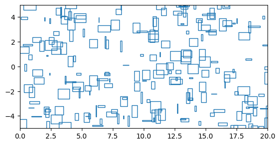
Here’s a close up, showing how some polygons overlap and some don’t:
gdf.plot(facecolor="none", edgecolor="tab:blue")
plt.xlim([0, 20])
plt.ylim([-5, 5])
(-5.0, 5.0)
Slow intersection finding
A brute-force method to find all intersecting polygons in this dataset would be to iterate through each row in the GeoDataFrame, checking all rows below that one for intersections. In each iteration, the subset of intersecting rows is captured as a separate GeoDataFrame and appended to a list. GeoPandas supplies a method intersects that can be used on a GeoSeries, which is like a pandas Series or column, but contains spatial datatypes called geometries. Here this is used on the geometry column which has index 4:
intersection_list = []
for ix, row in tqdm(gdf.iterrows()):
    intersection_gdf = gdf.iloc[(ix+1):][gdf.iloc[ix+1:, 4].intersects(gdf.iloc[ix, 4])]
    intersection_gdf['index_intersected'] = ix
    try:
        intersection_list.append(intersection_gdf)
    except:
        #No intersections
        pass
50000it [01:10, 711.65it/s]
These results can be combined into a GeoDataFrame, where the number of rows is the number of intersections:
pd.concat(intersection_list)
| bbox_lon_min | bbox_lon_max | bbox_lat_min | bbox_lat_max | geometry | index_intersected | |
|---|---|---|---|---|---|---|
| 465 | -47.544003 | -47.482310 | 50.534371 | 50.913198 | POLYGON ((-47.544 50.53437, -47.48231 50.53437... | 0 |
| 9595 | -47.330469 | -47.326180 | 50.411872 | 50.771513 | POLYGON ((-47.33047 50.41187, -47.32618 50.411... | 0 |
| 31584 | 147.397633 | 148.310990 | -5.486488 | -4.705461 | POLYGON ((147.39763 -5.48649, 148.31099 -5.486... | 1 |
| 21631 | 73.650220 | 74.490801 | -53.122555 | -52.795703 | POLYGON ((73.65022 -53.12255, 74.4908 -53.1225... | 2 |
| 1520 | -154.509087 | -153.734553 | -67.132524 | -66.845929 | POLYGON ((-154.50909 -67.13252, -153.73455 -67... | 6 |
| ... | ... | ... | ... | ... | ... | ... |
| 49664 | 85.777778 | 86.265469 | -24.767249 | -24.459444 | POLYGON ((85.77778 -24.76725, 86.26547 -24.767... | 49278 |
| 49661 | -29.854836 | -29.110292 | 71.209361 | 71.422139 | POLYGON ((-29.85484 71.20936, -29.11029 71.209... | 49283 |
| 49543 | -104.701379 | -103.983279 | -83.056904 | -82.093236 | POLYGON ((-104.70138 -83.0569, -103.98328 -83.... | 49368 |
| 49922 | -173.759994 | -173.177144 | 54.214183 | 54.769436 | POLYGON ((-173.75999 54.21418, -173.17714 54.2... | 49398 |
| 49992 | 15.277091 | 16.213651 | 64.108388 | 64.361987 | POLYGON ((15.27709 64.10839, 16.21365 64.10839... | 49849 |
22880 rows × 6 columns
This indicates there are 22,880 intersections between polygons in the dataset. The numerical index of this GeoDataFrame can be compared with the index_intersected column to see which geometries intersect with each other.
Fast intersection finding
The brute-force method does not fully leverage the spatial index that underlies the geometry column of a GeoDataFrame. Roughly speaking, the spatial index uses an R-tree to group nearby objects in a data structure, so that the intersection checking procedure does not need to consider far-away geometries, only intersection candidates from nearby. The effect of this is that fewer candidates for any particular polygon need to be examined, reducing computation time. Here’s an example R-tree from the Wikipedia article, for visual intuition:

Image credit: By Skinkie, w:en:Radim Baca - Own work, Public Domain, https://commons.wikimedia.org/w/index.php?curid=9938400
GeoPandas sjoin operates on GeoDataFrames and can take a variety of predicates which describe spatial relationships between geometries, such as intersects. To find intersections within one dataset, spatially join it to itself:
%%time
intersection_gdf = gdf.sjoin(
    gdf,
    how='inner',
    predicate='intersects',
    lsuffix='left',
    rsuffix='right'
)
CPU times: user 71.1 ms, sys: 4.03 ms, total: 75.1 ms
Wall time: 74.2 ms
intersection_gdf.info()
<class 'geopandas.geodataframe.GeoDataFrame'>
Index: 95760 entries, 0 to 49999
Data columns (total 10 columns):
 #   Column              Non-Null Count  Dtype
---  ------              --------------  -----
 0   bbox_lon_min_left   95760 non-null  float64
 1   bbox_lon_max_left   95760 non-null  float64
 2   bbox_lat_min_left   95760 non-null  float64
 3   bbox_lat_max_left   95760 non-null  float64
 4   geometry            95760 non-null  geometry
 5   index_right         95760 non-null  int64
 6   bbox_lon_min_right  95760 non-null  float64
 7   bbox_lon_max_right  95760 non-null  float64
 8   bbox_lat_min_right  95760 non-null  float64
 9   bbox_lat_max_right  95760 non-null  float64
dtypes: float64(8), geometry(1), int64(1)
memory usage: 8.0 MB
The raw output includes some of the geometric information from the left and right GeoDataFrames, which in this case are the same GeoDataFrame gdf. Both index values of the resulting GeoDataFrame intersection_gdf and the values in the column index_right are taken from the index of gdf. These pairs of index values show which polygons from this dataset intersect with each other:
intersection_gdf['index_right'].head()
0     9595
0        0
0      465
1        1
1    31584
Name: index_right, dtype: int64
Unlike in the brute-force approach where each polygon was only checked once against all other polygons, here every polygon in the dataset has been compared with every other polygon twice, as well as itself, since a self-join was done. Remove rows where the GeoDataFrame index equals index_right, the index of the intersecting polygon, since these are intersections of a polygon with itself:
same_polygon = intersection_gdf.index == intersection_gdf['index_right']
intersection_gdf = intersection_gdf[~same_polygon]
intersection_gdf.shape
(45760, 10)
After getting rid of these vacuously true intersections, the number of rows here is still twice as many as the number of intersections. For example, the polygon with index 0 intersects with two others: indices 9595 and 465:
intersection_gdf['index_right'].head()
0     9595
0      465
1    31584
2    21631
6    27084
Name: index_right, dtype: int64
And vice versa: polygons with indices 9595 and 465 are reported as intersecting with index 0.
intersection_gdf.loc[intersection_gdf.index==9595, 'index_right']
9595    0
Name: index_right, dtype: int64
intersection_gdf.loc[intersection_gdf.index==465, 'index_right']
465    0
Name: index_right, dtype: int64
To get rid of duplicates like this, make the index into a column to more easily work with it, then make a new column index_min_max which is the left and right indices of the intersecting polygons, but sorted as a comma-separated list:
intersection_gdf['index_left'] = intersection_gdf.index

intersection_gdf['index_min_max'] = (
    intersection_gdf[['index_left', 'index_right']].min(axis=1).astype(str).str.cat(
        intersection_gdf[['index_left', 'index_right']].max(axis=1).astype(str),
        sep=', '
    )
)
index_min_max will be identical for an intersection no matter which of the two polygons is in the index or index_right column, and can be used to deduplicate the dataset. By supplying keep='first' to pandas drop_duplicates, the record that is retained will have the smaller intersecting index in the GeoDataFrame index, and the larger intersecting index in the index_right column, since the GeoDataFrame intersection_gdf was sorted on its index to begin with.
print(intersection_gdf.shape)
intersection_gdf.drop_duplicates(subset='index_min_max', keep='first', inplace=True)
print(intersection_gdf.shape)
(45760, 12)
(22880, 12)
After this 22,880 intersections are found, as in the brute-force approach. It takes a little extra coding effort to tease apart the results of the spatial self-join, but this becomes worth it as datasets grow larger and the time difference in processing between the two approaches grows. In this synthetic example 50,000 polygons are used, which took a little over a minute in the slow approach and less than a second in the fast approach. I tried with several other numbers of polygons and found the following processing times for the slow and fast approaches:
time_compare_df = pd.DataFrame(
    data={'Number of polygons':[5000, 50000, 100000, 200000],
          'Slow intersection finding':[4, 70, 215, 717],
          'Fast intersection finding':[0.017, 0.104, 0.223, 0.746]
         }
).set_index('Number of polygons')
time_compare_df
| Slow intersection finding | Fast intersection finding | |
|---|---|---|
| Number of polygons | ||
| 5000 | 4 | 0.017 |
| 50000 | 70 | 0.104 |
| 100000 | 215 | 0.223 |
| 200000 | 717 | 0.746 |
time_compare_df.plot(marker='x')
plt.ylabel('Seconds')
Text(0, 0.5, 'Seconds')
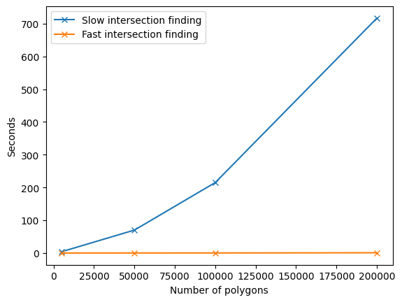
Real-world polygons representing field boundaries are often more complicated than the simple rectangles constructed here, and it can take hours or days to process similar numbers of polygons for intersections using the brute force approach. The benefits of a spatial index are even more valuable in this situation.
Fast intersection within buffer
sjoin_nearest is similar to sjoin, but matches geometries based on distance within some limit. The approach of doing a self-join can be extended to sjoin_nearest to determine which polygons within a single dataset are within a certain distance of each other.
With this intersection-finding method, a maximum search distance is supplied, so the GeoDataframe needs to be in a projected Coordinate Reference System in units of distance and not degrees. ESRI:54034 is a cylindrical equal area projection for the world:
gdf_projected = gdf.to_crs('ESRI:54034')
sjoin_nearest may be called as a method on a GeoDataframe. The differences from sjoin include specifying the maximum distance max_distance within which to search for geometries in the right GeoDataframe. The units are the same as the Coordinate Reference System, which are meters in this case. Unlike with sjoin, here the opportunity exists to automatically exclude intersections with identical geometries, by supplying exclusive=True. This spatial self-join looks for all geometries within a dataset that are within 10 km of each other, excluding the fact that a geometry is within 10 km of itself:
%%time
intersection_nearest_gdf = gdf_projected.sjoin_nearest(
    right=gdf_projected,
    how='inner',
    max_distance=10000,
    lsuffix='left',
    rsuffix='right',
    distance_col=None,
    exclusive=True
)
intersection_nearest_gdf.info()
<class 'geopandas.geodataframe.GeoDataFrame'>
Index: 53438 entries, 0 to 49997
Data columns (total 10 columns):
 #   Column              Non-Null Count  Dtype
---  ------              --------------  -----
 0   bbox_lon_min_left   53438 non-null  float64
 1   bbox_lon_max_left   53438 non-null  float64
 2   bbox_lat_min_left   53438 non-null  float64
 3   bbox_lat_max_left   53438 non-null  float64
 4   geometry            53438 non-null  geometry
 5   index_right         53438 non-null  int64
 6   bbox_lon_min_right  53438 non-null  float64
 7   bbox_lon_max_right  53438 non-null  float64
 8   bbox_lat_min_right  53438 non-null  float64
 9   bbox_lat_max_right  53438 non-null  float64
dtypes: float64(8), geometry(1), int64(1)
memory usage: 4.5 MB
CPU times: user 1.06 s, sys: 352 ms, total: 1.41 s
Wall time: 1.03 s
intersection_nearest_gdf['index_right'].head()
0     9595
0      465
1    31584
2    21631
3    11176
Name: index_right, dtype: int64
Similar to the results of sjoin, every intersection is listed twice here, so the number of unique intersections is half the dataframe row count:
intersection_nearest_gdf.shape[0]/2
26719.0
This is more intersections than when not using a buffer (22,880), which makes sense.
Conclusion and further resources
This post showed how to use sjoin and sjoin_nearest to perform spatial self-joins in GeoPandas, to efficiently find overlaps within a geographic dataset. The efficiency gains over a slower, brute-force method become more apparent as the size of datasets grow, and the geographic data is more complex.
The spatial join methods shown here were illustrated with self-joins, but could be extended to work with two different datasets, to answer questions like “how many homes in this city are within 2 miles of a grocery store?” with a homes dataset and a grocery store dataset.
These analyses performed in a Python environment with GeoPandas could also be performed in SQL databases that offer support for spatial datatypes. PostGIS/PostgreSQL is typically the first-choice SQL platform when working with spatial data is important - spatial datatypes are also available in MySQL.
While a massive speed boost was observed here by spatially joining a dataset on itself, it has also been shown that if the spatial extent of two geographic datasets is similar or the same, it may be faster to break one of them up into smaller sections, and iterate through a spatial join with each of these.