Overfitting, underfitting, and the bias-variance tradeoff
Overfitting, underfitting, and the bias-variance tradeoff are foundational concepts in machine learning. A model is overfit if performance on the training data, used to fit the model, is substantially better than performance on a test set, held out from the model training process. For example, the prediction error of the training data may be noticeably smaller than that of the testing data. Comparing model performance metrics between these two data sets is one of the main reasons that data are split for training and testing. This way, the model’s capability for predictions with new, unseen data can be assessed.
When a model overfits the training data, it is said to have high variance. One way to think about this is that whatever variability exists in the training data, the model has “learned” this very well. In fact, too well. A model with high variance is likely to have learned the noise in the training set. Noise consists of the random fluctuations, or offsets from true values, in the features (independent variables) and response (dependent variable) of the data. Noise can obscure the true relationship between features and the response variable. Virtually all real-world data are noisy.
If there is random noise in the training set, then there is probably also random noise in the testing set. However, the specific values of the random fluctuations will be different than those of the training set, because after all, the noise is random. The model cannot anticipate the fluctuations in the new, unseen data of the testing set. This why testing performance of an overfit model is lower than training performance.
Overfitting is more likely in the following circumstances:
- There are a large number of features available, relative to the number of samples (observations). The more features there are, the greater the chance of discovering a spurious relationship between the features and the response.
- A complex model is used, such as deep decision trees, or neural networks. Models like these effectively engineer their own features, and have an opportunity develop more complex hypotheses about the relationship between features and the response, making overfitting more likely.
At the opposite end of the spectrum, if a model is not fitting the training data very well, this is known as underfitting, and the model is said to have high bias. In this case, the model may not be complex enough, in terms of the features or the type of model being used.
Let’s examine concrete examples of underfitting, overfitting, and the ideal that sits in between, by fitting polynomial models to synthetic data in Python.
#Import packages
import numpy as np #numerical computation
import matplotlib.pyplot as plt #plotting package
#Next line helps with rendering plots
%matplotlib inline
import matplotlib as mpl #additional plotting functionality
Underfitting and overfitting with polynomial models
First, we create the synthetic data. We:
- Choose 20 points randomly on the interval [0, 11). This includes 0 but not 11, technically speaking.
- Sort them so that they’re in order.
- Put them through a quadratic transformation and add some noise: \(y = (-x+2)(x-9) + \epsilon\).
- \(\epsilon\) is normally distributed noise with mean 0 and standard deviation 3.
Then we make a scatter plot of the data.
np.random.seed(seed=9)
n_points = 20
x = np.random.uniform(0, 11, n_points)
x = np.sort(x)
y = (-x+2) * (x-9) + np.random.normal(0, 3, n_points)
mpl.rcParams['figure.dpi'] = 400
plt.scatter(x, y)
plt.xticks([])
plt.yticks([])
plt.ylim([-20, 20])
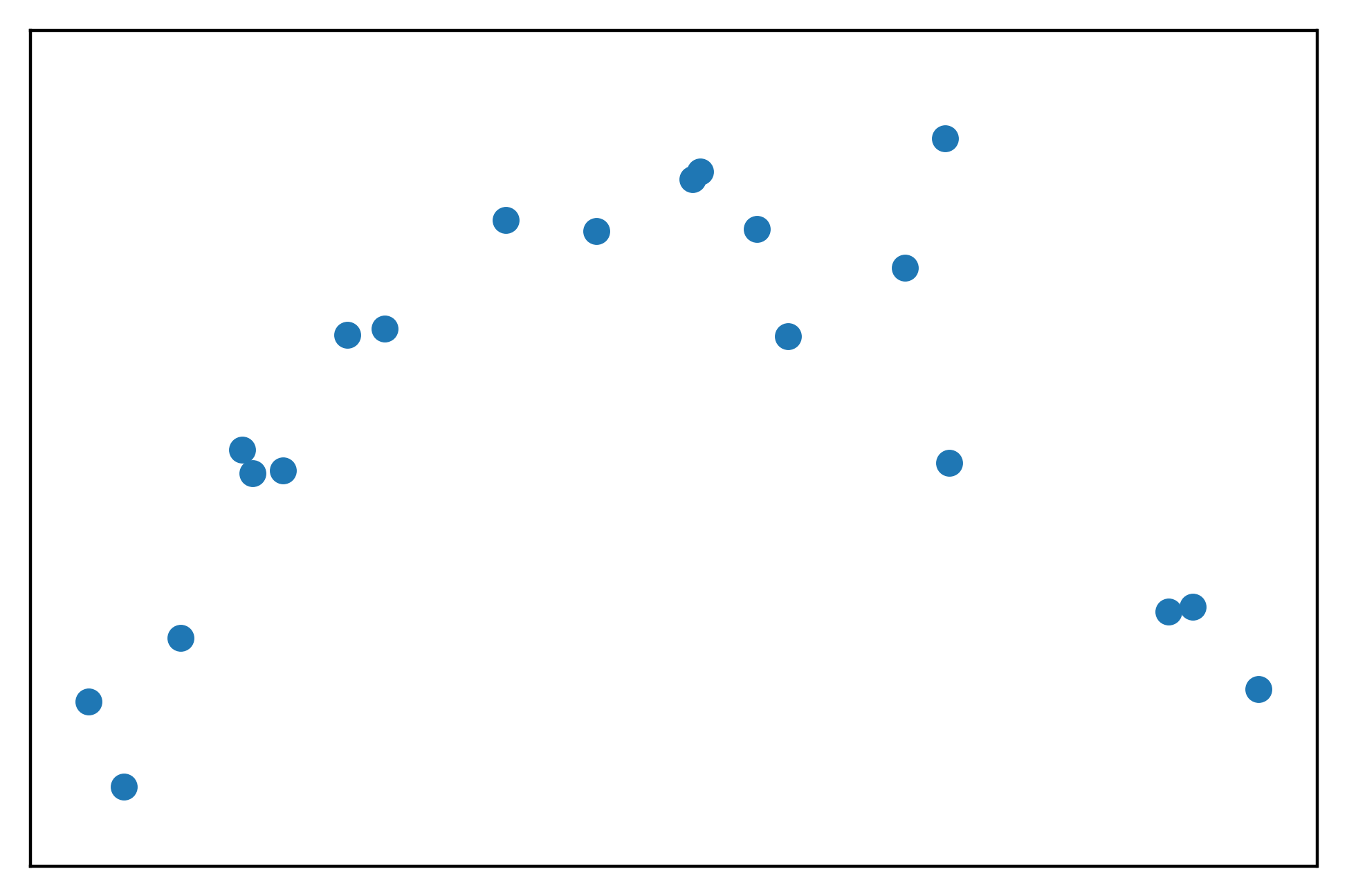
This looks like the shape of a parabola, as expected for a quadratic transformation of \(x\). However we can see the noise in the fact that not all the points appear that they would lie perfectly on the parabola.
In our synthetic example, we know the data generating process: the response variable \(y\) is a quadratic transformation of the feature \(x\). In general, when building machine learning models, the data generating process is not known. Instead, several candidate features are proposed, a model is proposed, and an exploration is made of how well these features and this model can explain the data.
In this case, we would likely plot the data, observe the apparent quadratic relationship, and use a quadratic model. However, for the sake of illustration of an underfit model, what does a linear model for these data look like?
We can fit a polynomial model of degree 1, in other words a linear model, with numpy’s polyfit:
lin_fit = np.polyfit(x, y, 1)
lin_fit
array([ 0.44464616, -0.61869372])
This has produced the slope and intercept of the line of best fit for these data. Let’s plot it and see what it looks like. We can calculate the linear transformation of the feature \(x\) using the slope and intercept we got from fitting the linear model, again using numpy, this time the polyval function. We’ll label this the “Underfit model”.
cmap = mpl.cm.get_cmap('tab10')
plt.scatter(x, y, label='Data', color=cmap(0))
plt.plot(x, np.polyval(lin_fit, x), label='Underfit model', color=cmap(1))
plt.legend(loc=[0.17, 0.1])
plt.xticks([])
plt.yticks([])
plt.ylim([-20, 20])
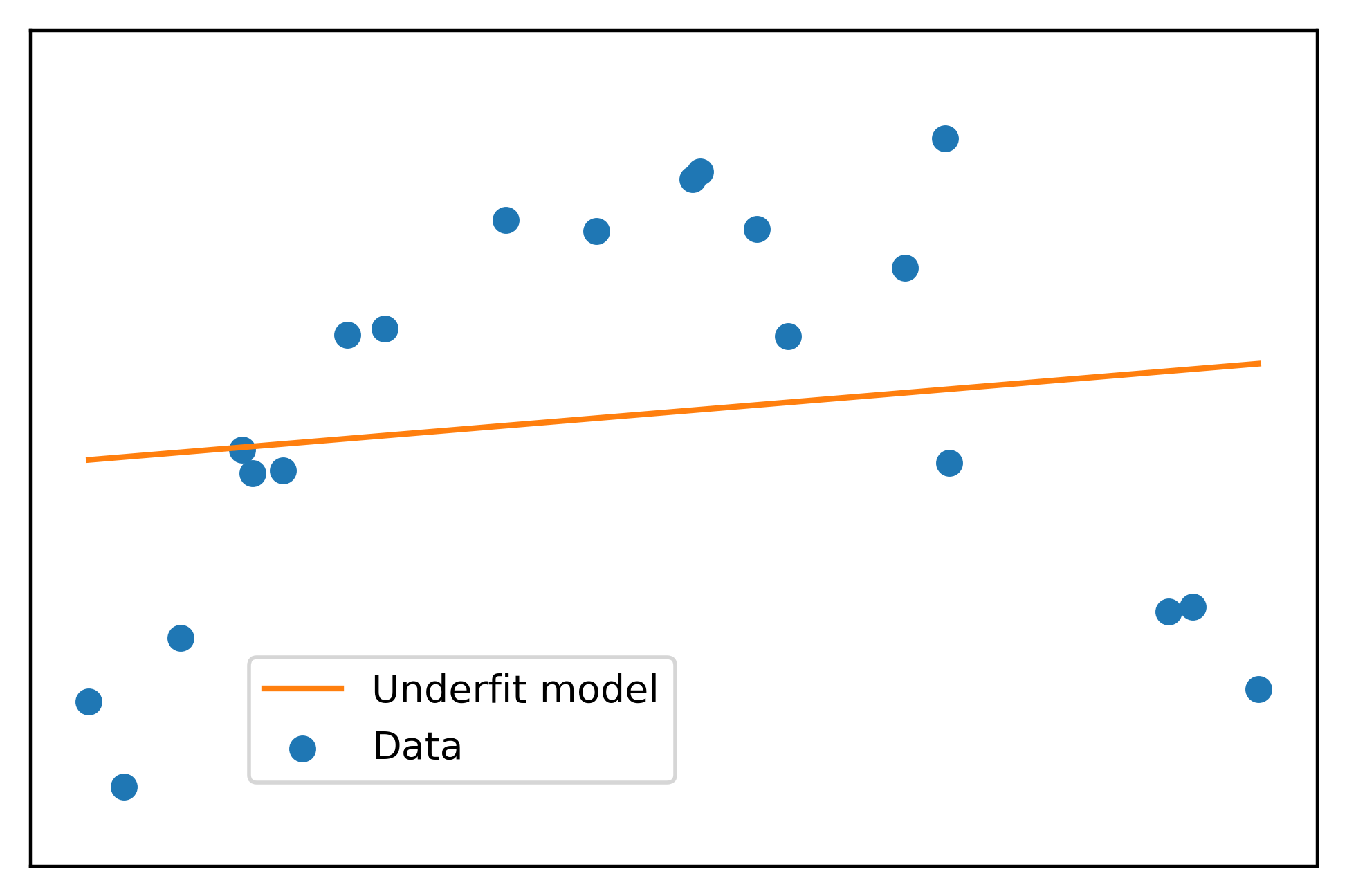
Doesn’t look like a very good fit, does it!
Now let’s imagine we have many features available, that are polynomial transformations of \(x\), specifically \(x^2\), \(x^3\),… \(x^{15}\). This would be a large amount of features relative to the amount of samples (20) that we have. Again, in “real life”, we probably wouldn’t consider a model with all these features, since by observation we can see that a quadratic model, or 2nd degree polynomial, would likely be sufficient. However, identifying the ideal features isn’t always so straightforward. Our illustrative example serves to show what happens when we are very clearly using too many features.
Let’s make a 15 degree polynomial fit:
high_poly_fit = np.polyfit(x, y, 15)
high_poly_fit
array([ 1.04191511e-05, -7.58239114e-04,  2.48264043e-02, -4.83550912e-01,
        6.24182399e+00, -5.63097621e+01,  3.64815913e+02, -1.71732868e+03,
        5.87515347e+03, -1.44598953e+04,  2.50562989e+04, -2.94672314e+04,
        2.21483755e+04, -9.60766525e+03,  1.99634019e+03, -1.43201982e+02])
These are the coefficients of all the powers of \(x\) from 1 through 15 in this model, and the intercept. Notice the widely different scales of the coefficients: some are close to zero, while others are fairly large in terms of magnitude (absolute value). Let’s plot this model as well. First we generate a large number of evenly spaced points over the range of \(x\) values, so we can see how this model looks not only for the particular values of \(x\) used for model training, but also for values in between.
curve_x = np.linspace(0,11,333)
plt.scatter(x, y, label='Data', color=cmap(0))
plt.plot(x, np.polyval(lin_fit, x), label='Underfit model', color=cmap(1))
plt.plot(curve_x, np.polyval(high_poly_fit, curve_x),
         label='Overfit model', color=cmap(2))
plt.legend(loc=[0.17, 0.1])
plt.xticks([])
plt.yticks([])
plt.ylim([-20, 20])
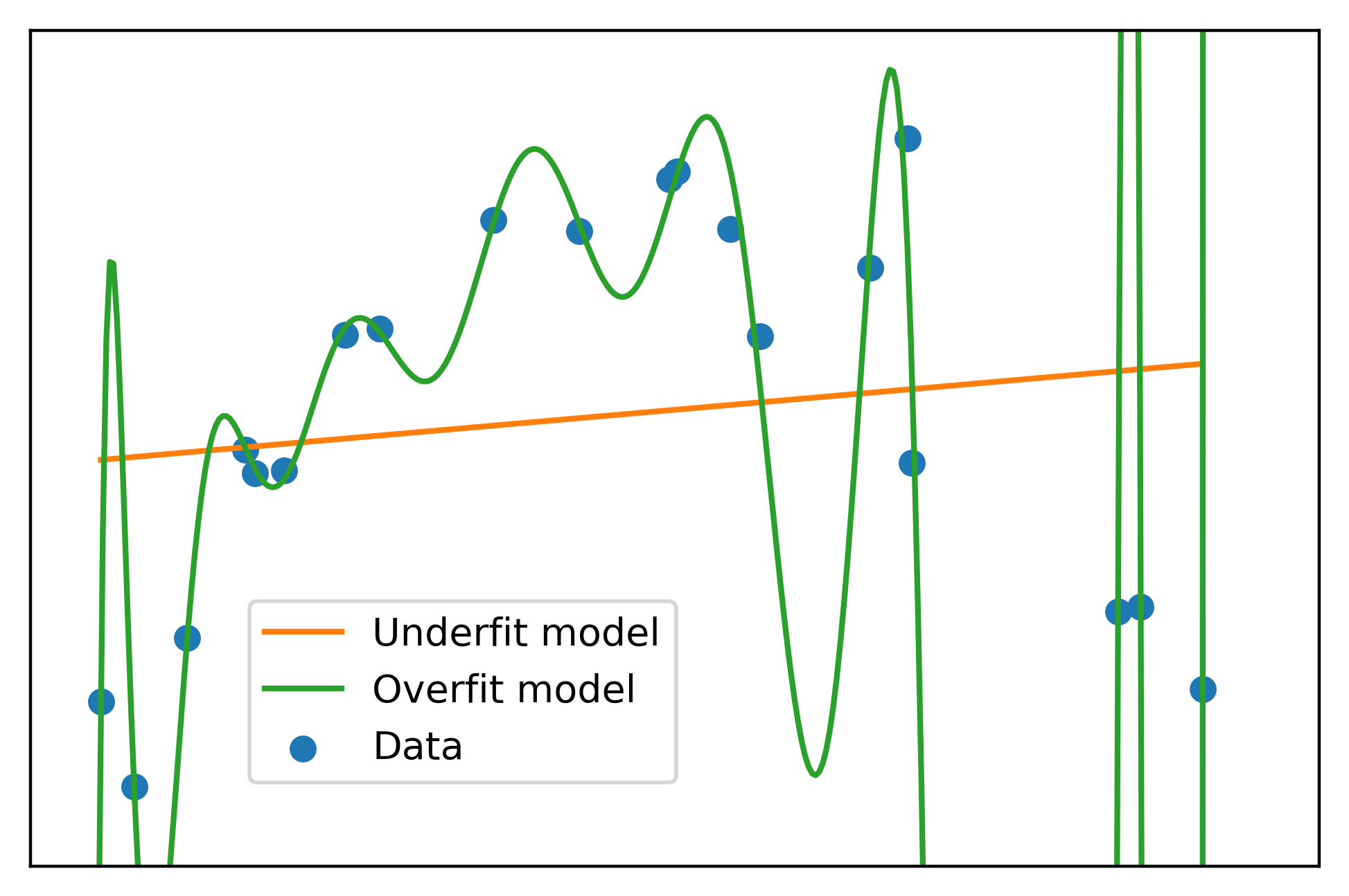
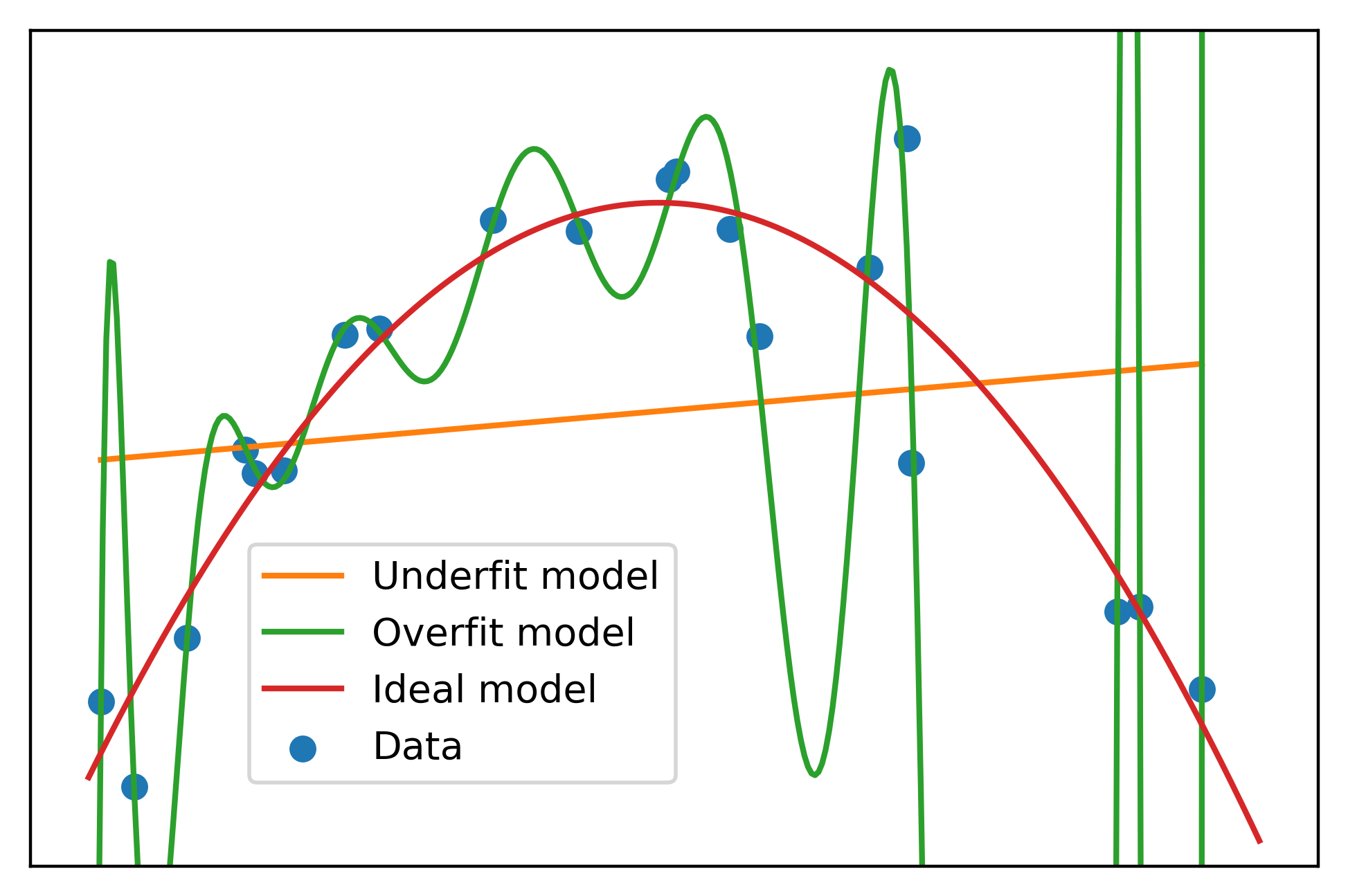
This is a classic case of overfitting. The overfit model passes nearly perfectly through all the training data. However it’s easy to see that for values in between, the overfit model does not look like a realistic representation of the data generating process. Rather, the overfit model has become tuned to the noise of the training data. This matches the definition of high variance given above.
In this last graph, you can see another definition of high variance: a small change in the input \(x\) can result in a large change in the output \(y\).
Further, you can imagine that if we generated a new, larger synthetic data set, using the same quadratic function \(y = (-x+2)(x-9)\), but added new randomly generated noise \(\epsilon\) according to the same distribution we used above, then randomly sampled 20 points and fit the high-degree polynomial, the resulting model would look much different. It would pass almost perfectly through these new noisy points and the coefficients of the 15 degree polynomial would be very different to allow this to happen. Repeating this process with different samples of 20 points, would continue to result in highly variable coefficient estimates. In other words, the coefficients would have high variance between samples of the data used for model training. This is yet another definition of a model with high variance.
With our synthetic data, since in this case we know the data generating process, we can see how a 2nd degree polynomial fit looks in comparison with the underfit and overfit models.
plt.scatter(x, y, label='Data', color=cmap(0))
plt.plot(x, np.polyval(lin_fit, x), label='Underfit model', color=cmap(1))
plt.plot(curve_x, np.polyval(high_poly_fit, curve_x),
         label='Overfit model', color=cmap(2))
plt.plot(curve_x, np.polyval(np.polyfit(x, y, 2), curve_x),
         label='Ideal model', color=cmap(3))
plt.legend(loc=[0.17, 0.1])
plt.xticks([])
plt.yticks([])
plt.ylim([-20, 20])
That’s more like it. But what do we do in the real world, when we’re not using made-up data, and we don’t know the data generating process? There are a number of machine learning techniques to deal with overfitting. One of the most popular is regularization.
Regularization with ridge regression
In order to show how regularization works to reduce overfitting, we’ll use the scikit-learn package. First, we need to create polynomial features manually. While above we simply had to tell numpy to fit a 15 degree polynomial to the data, here we need to manually create the features \(x^2\), \(x^3\),… \(x^{15}\) and then fit a linear model to find their coefficients. Scikit-learn makes creating polynomial features easy with PolynomialFeatures. We just say we want 15 degrees worth of polynomial features, without a bias feature (intercept), then pass our array \(x\) reshaped as a column.
from sklearn.preprocessing import PolynomialFeatures
poly = PolynomialFeatures(degree=15, include_bias=False)
poly_features = poly.fit_transform(x.reshape(-1, 1))
poly_features.shape
(20, 15)
We get back 15 columns, where the first column is \(x\), the second \(x^2\), etc. Now we need to determine coefficients for these polynomial features. Above, we did this by using numpy to find the coefficients that provided the best fit to the training data. However, we saw this led to an overfit model. Here, we will pass these data to a routine for ridge regression, which is a kind of regularized regression. Without going too far in to details, regularized regression works by finding the coefficients resulting in the best fit to the data while also limiting the magnitude of the coefficients.
The effect of this is to provide a slightly worse fit to the data, in other words a model with higher bias. However, the goal is to avoid fitting the random noise, thus eliminating the high variance issue. Therefore, we are hoping to trade some variance for some bias, to obtain a model of the signal and not the noise.
We will use the Ridge class from scikit-learn to do a ridge regression.
from sklearn.linear_model import Ridge
ridge = Ridge(alpha=0.001, fit_intercept=True, normalize=True,
                        copy_X=True, max_iter=None, tol=0.001,
                        random_state=1)
There are many options to set when instantiating the Ridge class. An important one is alpha. This controls how much regularization is applied; in other words, how strongly the coefficient magnitudes are penalized, and kept close to zero. We will use a value determined from experimentation just to illustrate the process. In general, the procedure for selecting alpha is to systematically evaluate a range of values, by examining model performance on a validation set or with a cross-validation procedure, to determine which one is expected to provide the best performance on the unseen test set. alpha is a model hyperparameter and this would be the process of hyperparameter tuning.
The other options we specified for Ridge indicate that we’d like to fit an intercept, normalize the features to the same scale before model fitting, which is necessary since the coefficients will all be penalized in the same way, and a few others. I’m glossing over these details here, although you can consult the scikit-learn documentation, as while as my book, for further information.
Now we proceed to fit the ridge regression using the polynomial features and the response variable.
ridge.fit(poly_features, y)
Ridge(alpha=0.001, copy_X=True, fit_intercept=True, max_iter=None,
   normalize=True, random_state=1, solver='auto', tol=0.001)
What do the values of the fitted coefficients look like, in comparison to those found above by fitting the polynomial with numpy?
ridge.coef_
array([ 8.98768521e+00, -5.14275445e-01, -3.95480123e-02, -1.10685070e-03,
        4.49790120e-05,  8.58383048e-06,  6.74724995e-07,  3.02757058e-08,
       -3.81325130e-10, -2.54650509e-10, -3.25677313e-11, -2.66208560e-12,
       -1.05898398e-13,  1.22711353e-14,  3.90035611e-15])
We can see that the coefficient values from the regularized regression are relatively small in magnitude, compared to those from the polynomial fit. This is how regularization works: by “shrinking” coefficient values toward zero. For this reason regularization may also be referred to as shrinkage.
Let’s obtain the predicted values y_pred over the large number of evenly spaced points curve_x we used above, for plotting. First we need to generate the polynomial features for all these points.
poly_features_curve = poly.fit_transform(curve_x.reshape(-1, 1))
y_pred = ridge.predict(poly_features_curve)
We’ll remove the underfit model from our plot, and add the regularized model.
plt.scatter(x, y, label='Data', color=cmap(0))
plt.plot(curve_x, np.polyval(high_poly_fit, curve_x),
         label='Overfit model', color=cmap(2))
plt.plot(curve_x, np.polyval(np.polyfit(x, y, 2), curve_x),
         label='Ideal model', color=cmap(3))
plt.plot(curve_x, y_pred,
         label='Regularized model',color=cmap(4), linestyle='--')
plt.legend(loc=[0.17, 0.1])
plt.xticks([])
plt.yticks([])
plt.ylim([-20, 20])
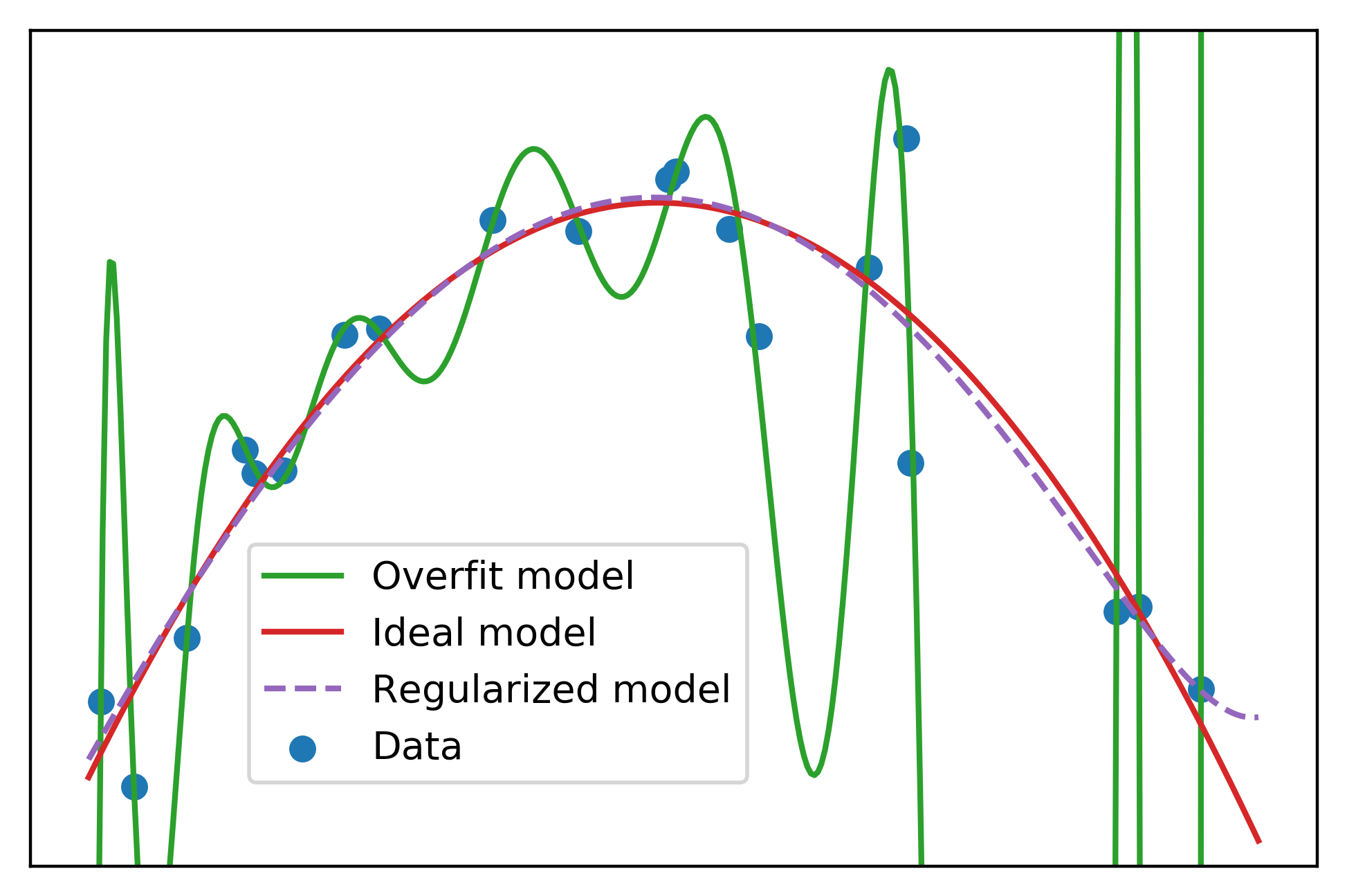
The regularized model looks similar to the ideal model. This shows that even if we don’t have knowledge of the data generating process, as we typically don’t in real-world predictive modeling work, we can still use regularization to reduce the effect of overfitting when a large number of candidate features are available.
Note, however, that the regularized model should not be used for extrapolation. We can see that the regularized model starts to increase toward the right side of the plot. This increase should be viewed with suspicion, as there is nothing in the training data that makes it clear that this would be expected. This is an example of the general view that extrapolation of model predictions outside the range of the training data is not recommended.
Effect of regularization on model testing performance
The goal of trading variance for bias is to improve model performance on unseen testing data. Let’s generate some testing data, in the same way we generated the training data, to see if we achieved this goal. We repeat the process used to generate \(x\) and \(y = (-x+2)(x-9) + \epsilon\) above, but with a different random seed. This results in different points \(x\) over the same interval and different random noise \(\epsilon\) from the same distribution, creating new values for the response variable \(y\), but from the same data generating process.
np.random.seed(seed=4)
n_points = 20
x_test = np.random.uniform(0, 11, n_points)
x_test = np.sort(x_test)
y_test = (-x_test+2) * (x_test-9) + np.random.normal(0, 3, n_points)
We’ll also define a lambda function to measure prediction error as the root mean squared error (RMSE).
RMSE = lambda y, y_pred: np.sqrt(np.mean((y-y_pred)**2))
What is the RMSE of our first model, the polynomial fit to the training data?
y_train_pred = np.polyval(high_poly_fit, x)
RMSE(y, y_train_pred)
1.858235982416223
How about the RMSE on the newly generated testing data?
y_test_pred = np.polyval(high_poly_fit, x_test)
RMSE(y_test, y_test_pred)
9811.219078261804
The testing error is vastly larger than the training error from this model, a clear sign of overfitting. How does the regularized model compare?
y_train_pred = ridge.predict(poly_features)
RMSE(y, y_train_pred)
3.235497045896461
poly_features_test = poly.fit_transform(x_test.reshape(-1, 1))
y_test_pred = ridge.predict(poly_features_test)
RMSE(y_test, y_test_pred)
3.5175193708774946
While the regularized model has a bit higher training error (higher bias) than the polynomial fit, the testing error is greatly improved. This shows how the bias-variance tradeoff can be leveraged to improve model predictive capability.
Conclusion
This post illustrates the concepts of overfitting, underfitting, and the bias-variance tradeoff through an illustrative example in Python and scikit-learn. It expands on a section from my book Data Science Projects with Python: A case study approach to successful data science projects using Python, pandas, and scikit-learn. For a more in-depth explanation of how regularization works, how to use cross-validation for hyperparameter selection, and hands-on practice with these and other machine learning techniques, check out the book, which you can find on Amazon, with Q&A and errata here.
Here are a few final thoughts on bias and variance.
Statistical definitions of bias and variance: This post has focused on the intuitive machine learning definitions of bias and variance. There are also more formal statistical definitions. See this document for a derivation of the mathematical expressions for the bias-variance decomposition of squared error, as well as The Elements of Statistical Learning by Hastie et al. for more discussion of the bias-variance decomposition and tradeoff.
Countering high variance with more data: In his Coursera course Machine Learning, Andrew Ng states that, according to the large data rationale, training on a very large data set can be an effective way to combat overfitting. The idea is that, with enough training data, the difference between the training and testing errors should be small, which means reduced variance. There is an underlying assumption to this rationale, that the features contain sufficient information to make accurate predictions of the response variable. If not, the model will suffer from high bias (high training error), so the low variance would be a moot point.
A little overfitting may not be a problem: Model performance on the testing set is often a bit lower than on the training set. We saw this with our regularized model above. Technically, there is at least a little bit of overfitting going on here. However, it may not matter, since the best model is usually considered to be that with the highest testing score.