Why decision trees are more flexible than linear models
This blog post will examine a hypothetical dataset of website visits and customer conversion, to illustrate how decision trees are a more flexible mathematical model than linear models such as logistic regression.
Introduction
Imagine you are monitoring the webpage of one of your products. You are keeping track of how many times individual customers visit this page, the total amount of time they’ve spent on the page across all their visits, and whether or not they bought the product. Your goal is to be able to predict, for future visitors, how likely they are to buy the product, based on the page visit data. You are considering presenting a discount, or some other kind of offer, to customers you think are likely to buy the product but haven’t yet.
After logging the data on many customers, you visualize them and see the following, including some jitter to help see all the data points:
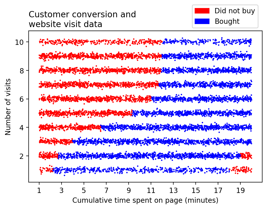
There are several interesting patterns visible here. We see that in general, the longer someone spends on the page, the more likely they are to purchase the item. However, this effect seems to depend on the number of visits, in a complex way. Someone who visited the page once and spent at least two minutes there (i.e. two minutes per visit) seems likely to buy, at least up until 18 or so minutes. But someone who visited 10 times as much as this seems likely to buy after only 12 minutes cumulative time (1.2 minutes per visit).
Additionally, there is a phenomenon of customers who spend a relatively long time (at least 18 or 19 minutes) over a relatively small number of visits (just one or two), who don’t buy. Maybe they opened the page, but then walked away from their computer, and closed the page as soon as they came back.
Whatever the reason, the patterns in this data set are interesting and complicated. If you want to create a predictive model of these data, you should consider the likely success of non-linear models, such as decision trees, versus linear models, such as logistic regression.
Logistic Regression as a linear model
At a high level, linear models will take the feature space (the two-dimensional space where time is on the x-axis and number of visits is on the y-axis, as in the graph above), and seek to draw a straight line somewhere that creates an accurate division of the two classes of the response variable (“Bought” or “Did not buy”).
Consider how well this will work. Where would you draw a straight line on the graph above, so that the two regions on either side of the line would contain responses of only one class?
It should be apparent that this would not be an entirely successful effort. The best you could probably do would be to draw a line that isolates non-buying customers who spent relatively little time on the page, represented by the region of dots to the left of the graph, from the blue dots representing buying customers to the right. While this would basically ignore the little group of customers to the lower right (few visits but a relatively long time), it’s the best overall for most customers, using the straight-line approach.
In fact, this is essentially what a logistic regression classifier looks like when the model is calibrated to these data.
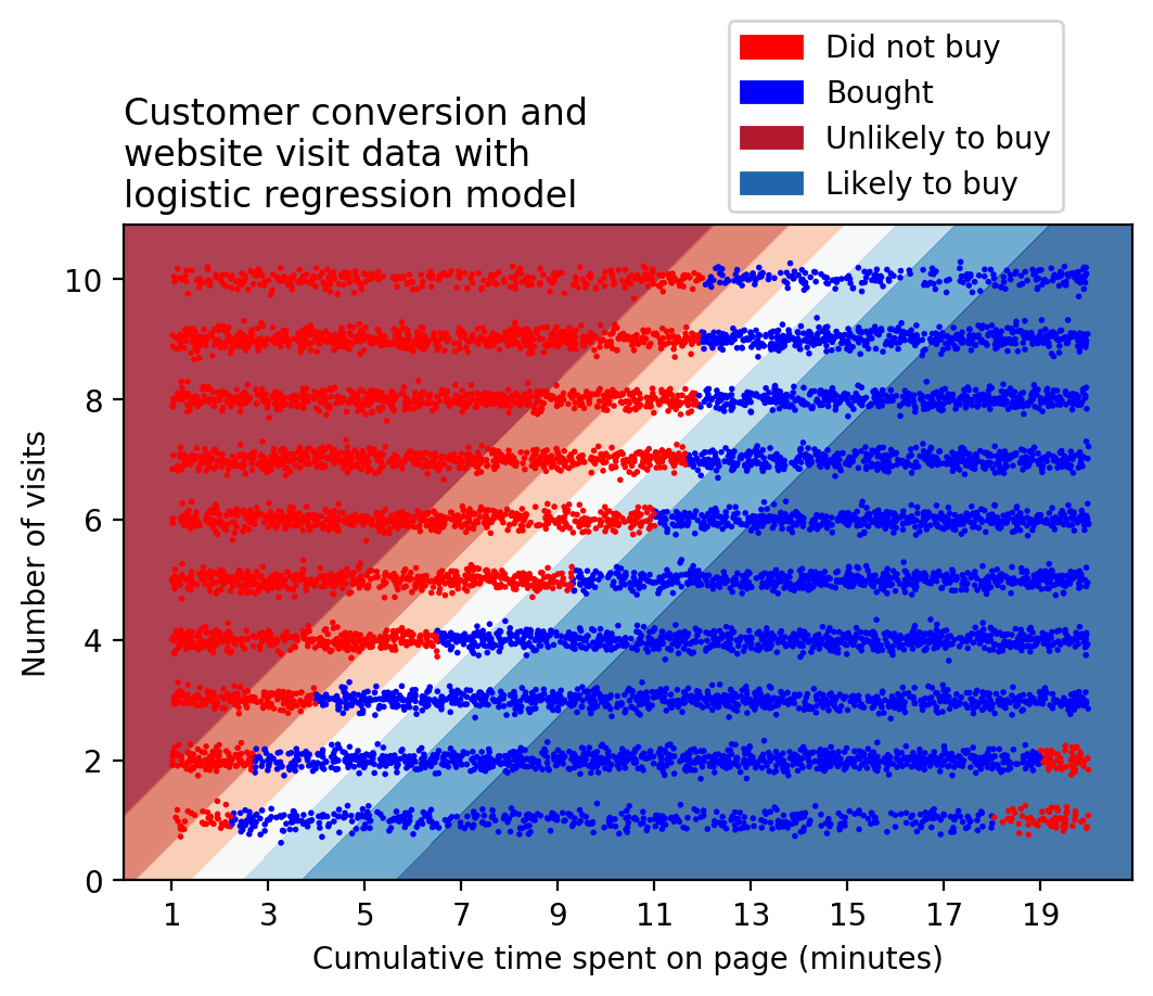
The above graph shows the regions of prediction (“Unlikely to buy” and “Likely to buy”) as red or blue shading in the background. Deeper colors indicate a higher likelihood for either class. The conceptual straight-line decision boundary that divides the two regions mentioned above, would run right through the white portion of the background, where the probability of belonging to either class is very low. In other words, the model is “uncertain” about what prediction to make in this region.
From the above graph, it can be seen that in addition to ignoring the small group of non-buying customers in the lower right, a straight line is also not a great model for isolating the non-buying customers on the left of the graph. While you can imagine that a more complex division, such as a curve, might be better able to define this boundary, a single straight line is not flexible enough.
Decision Trees as a non-linear model
How can we do better? Enter non-linear models. Decision trees are a prime example of non-linear models. Decision trees work by dividing the data in to regions based on “if-then” type of questions. For example, if a user spends less than three minutes over two or fewer visits, how likely are they to buy? Graphically, by asking many “if-then” questions, a decision tree can divide up the feature space using little segments of vertical and horizontal lines. This approach can create a more complex decision boundary, as shown below.
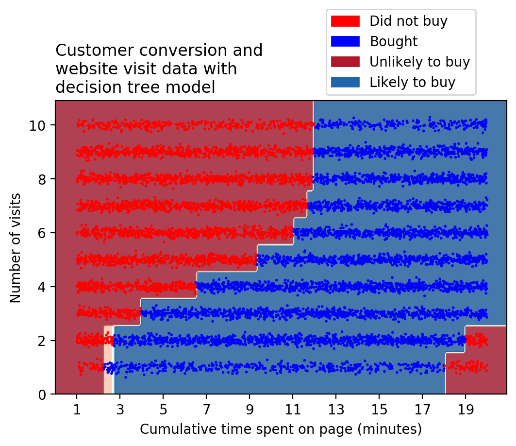
It should be clear that decision trees can be used with more success, to model this data set. Given this, you would have a better model for the likelihood of customer conversion and could then proceed to design offers to increase conversion.
Conclusion
This post has shown how non-linear models, such as decision trees, can more effectively describe relationships in complex data sets than linear models, such as logistic regression. It should be noted that linear models can be extended to non-linearity by various means including feature engineering. On the other hand, non-linear models may suffer from overfitting, since they are so flexible. Consequently, approaches to prevent decision trees from overfitting have been formulated using ensemble models such as random forests and gradient boosted trees, which are among the most successful machine learning techniques in use today. As a final caveat, note this blog post presents a hypothetical, synthetic data set, which can be modeled almost perfectly with decision trees. Real-world data is messier, but the same principles hold.
I hope you found this conceptual discussion helpful. For a more detailed explanation of how decision trees and logistic regression work “under the hood” with real-world data, and the python code for a similar hypothetical example to that shown here, check out my book Data Science Projects with Python.
Originally posted here